All published articles of this journal are available on ScienceDirect.

Automated Morphometric Analysis of the Femur on Large Anatomical Databases with Highly Accurate Correspondence Detection
Authors Info & Affiliations
Abstract
For a variety of medical applications, detailed knowledge on the statistical distribution of morphometric characteristics among specific patient groups is required. We present a novel approach for performing automated morphometric measurements on the surface of anatomical bone samples obtained from CT segmentation. The system developed supports various types of measurements (distances, angles, radii) on several kinds of features (points, lines, planes or circles), which are performed automatically for every bone sample in a given data set. The desired features can be specified by the user in two ways, either by marking them on a standardized template that is mapped to all samples via a correspondence mapping, or by hierarchically building new features from existing features.
The system was implemented and tested on a database containing about 1200 segmented femur. The quality of the automated matching was assessed through a study comparing the performance of the system with results obtained from manual labeling by medical experts. It was found that the deviation between the two methods was generally less than 2mm.
1. INTRODUCTION
With increase in storage capacity and processing power of computer systems, the gathering of anatomical data (CT, MRI, etc.) into centralized databases has found widespread adoption in commercial and academic settings. Many medical applications require a statistical analysis of the data based on patient-specific attributes (e.g. age, sex, ethnic group).
One exemplary area in which such findings are of high importance is implant design, where the shape and size of the implant have to be adapted to the anatomy of the target patient group as well as possible. Other examples include the tracking of epidemiological developments (e.g. increase in body height over time with respect to sex, ethnicity, etc.), tabulation of anatomical reference data (e.g. for use in planning deformity corrections), or application of various data mining techniques (e.g. predicting the risk of delivery complications based on specific anatomical features of the maternal pelvis).
The characteristics dealt with in this paper are quantities (distances, angles, radii) measured on anatomical features, such as “radius of the femoral head” or “angle between femoral shaft and neck axis”, etc. Traditionally, these kinds of measurements could only be obtained with high amounts of user interaction, being performed on MRI images [1], ultrasound imaging [2, 3] or through a variety of other means [4, 5]. However, the manual approach is very time consuming and has other drawbacks such as low reproducibility due to interandintrasubject variance. MRI or CT-based measurements are often performed on single slices, and thus disregard the 3D nature of the problem. Also, to be statistically meaningful, the desired measurements have to be performed on a sufficiently large number of specimens, which is very cumbersome when done manually. Ideally it should be easy to quickly change the input parameters of the evaluation (e.g. redefine the points between which a measurement is made).
These requirements call for an automated procedure to perform the measurements. Such a procedure would accept a specification of the quantity to be measured, and measure this quantity on every sample of an input data set. These measurements have to be done for every sample on its own rather than performing measurements on a samples’ mean because the arithmetic mean differs from the geometrical mean which is shown in Fig. (1). Once the results have been computed, they can be further analyzed with respect to their statistical properties. Also, if patient metadata (e.g. patient age, sex, height, weight, ethnic group, etc.) is stored along with the actual anatomical data, the evaluation can be constrained to a specific subset of the input. Thus, highly relevant results can be obtained (e.g. “CCD angle of Caucasian women older than 50 years”).
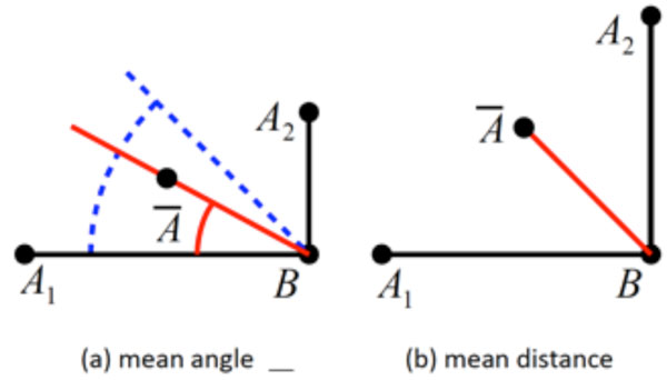
Given are two “shapes” (A1,B1) and (A2,B2), and their arithmetic mean with B1 = B2 = B = B. (a) The quantity to be measured is the angle α formed with the horizontal axis, with α1 = 0° and α2 = 90°. The correct mean angle, (blue) differs from the angle measured on the mean (red). (b) The quantity to be measured is the distance d(A,B) between A and B. The correct mean distance = d1 = d2 differs from the distance measured on the mean (red), with .
The main obstacle for the automation of this process lies in determining corresponding anatomical structures or landmarks on different samples. To produce meaningful results, the features involved in the measurements must be consistently identified on all members of the input set, a task that is complicated by the high interindividual variance of anatomical structures.
This paper presents an approach which addresses this problem. The proposed system identifies different kinds of features (explicitly defined landmarks as well as user-supplied point features) on segmented bone samples stored in a database, and performs measurements on these. The system works fully autonomously both during data preprocessing which has to be done once for every sample in the database, as well as during the actual evaluation, in which measurements specified by the user are performed on the bone samples. The system was implemented on a database containing several thousand femur samples. The quality of the anatomical registration was assessed through a study comparing point correspondences found by the automated system with points manually marked by medical experts.
2. BACKGROUND
Recently, a lot of research has gone into the generation of statistical shape models of bones which capture the statistical variance of a set of shapes [6]. Let a shape with n vertices be represented as a 3n element vector x = (x1,y1,z1,...,xn,yn,zn)T, and let {x1,...,xm} be a set of sample shapes which are affinely aligned (i.e. aligned with respect to rotation, translation and scaling), and whose vertices correspond (i.e. whose element vectors represent ordered sets of corresponding points). Then, each of the sample shapes can be expressed as
in which is the mean shape, Φ a matrix of eigenvectors of the covariance matrix of the data, and bi the weight vector of the i-th shape.These methods have a wide variety of applications, including modeling of bone shape for segmentation purposes [7], surgical planning [8] or even inter-species comparisons of long bones [9]. However, they model the variance of a shape “as a whole” and thus are not well suited for determining the statistical properties of morphometric quantities (e.g. “femur CCD angle”, “femur head radius”). The main reason is that the modes identified by the principal component analysis do not directly correspond to specific quantities, i.e. there is no eigenmode that uniquely controls the CCD angle or other types of quantities.
Also, it should be noted that the calculation of a mean shape alone is not sufficient for obtaining information about the distribution of a quantity. Apart from the fact that it does not provide any way for determining characteristics like standard deviation, median, etc., a quantity measured on the mean shape is not in general identical to the mean of the quantities measured on the samples (see Fig. 1 for an illustration of the problem).
The main obstacle in the generation of statistical shape models is the problem of determining corresponding point sets across all samples. Although the system proposed in this paper does not use a statistical shape model, it still requires a dense correspondence mapping for the samples. A large number of approaches exist for the automated determination of the mapping transformation, see [10-12]. One way to obtain dense mappings is to regard the correspondence finding problem as the registration task in which a template mesh is deformed until its surface matches that of a sample [13]. A widely used method to describe 3D deformations uses cubic B-Spline interpolation inside a control-point lattice [14] which provides smooth deformations
3. SYSTEM DESCRIPTION
The system performs measurements on segmented bone surfaces represented by a triangular mesh. This kind of surface representation can be generated from CT volume images through a variety of methods outside the scope of this paper [15, 16]. For the rest of this paper, we assume the availability of segmented surfaces, annotated with patient metadata.
The proposed system can measure quantities like lengths, angles and diameters. All measurements are based on features which can be points, lines, planes or circles. For example, an evaluation could measure the distance of a point from a line, or the angle between a line and a plane. During an evaluation the features involved are identified on every input sample, and the desired quantity is measured and recorded.
Two different kinds of features exist: correspondence features and derived features.
- Correspondence Features are features that are determined through correspondence mapping. Correspondence features are always “point” features although they can be used as building blocks for more complex types (see derived features). The user can define correspondence features by marking points on a template shape. During the evaluation, these features are mapped to their corresponding location on every sample.
- Derived Features are features that are constructed based on existing features (e.g. a plane (C1,C2,C3) defined by three correspondence points). They can be built hierarchically, i.e. derived features may serve as input to ”higher-level” derived features. Thus, complex geometric constructions can be specified (e.g. construct a line from the intersection of two planes, etc.).
3.1. Correspondence Features
Correspondences are found by having the user mark points on a template shape and then mapping these points to the samples during an evaluation. Fig. (2) displays the mapping result of two template points. Correspondence features are always points, but in combination with derived features the user can perform arbitrary measurements between corresponding parts of anatomy over the entire range of input samples.
Correspondence points, marked by the user on the template (left, blue) and mapped to a set of samples).
The mapping transformation from the template to the sample is precomputed for every specimen in the database. Once computed, it can be evaluated quickly at arbitrary points on the surface of the template. It yields a continuous, dense mapping.
The transformation here denoted as the function map(), maps a point xT on the template surface to the corresponding point on the sample xS. It uses for this mapping 3 more functions, namely affine(), deform() and surf() which are applied successively in the listed order. In detail:
- affine() is an affine transformation that aligns the template and the sample with respect to position, orientation and scaling,
- deform() is a non-rigid deformation mapping that deforms the template surface until it coincides with the sample,
- surf() maps a point to the closest surface point of the sample (which is necessary only because deform() is not fine-grained enough to capture small irregularities on the segmented surface).
The function map() can mathematically be written as the composition of these three constituent functions:
The affine transformation consists of scaling, rotation and translation. It is used to equilize the different coordinate systems of the template and the sample shape. The scaling is found through Procrustes analysis and necessary to compensate the different sizes of the samples compared to the template. The translational and rotational parts are obtained through a standard Iterative Closest Point (ICP) procedure, which is initialized with a transformation found through an analysis of the previously calculated anatomical features. For example, two femora are registered by aligning their shaft axes and coronal planes, and translating them until their centroids overlap. A similar procedure can be used for other kinds of bones.
The non-rigid deformation was implemented following the approach described in [17]. The template shape is embedded into a 3D deformation lattice, which is a regular grid whose vertices are control points that can be displaced, thereby controlling the deformation. The displacement of points inside the grid is interpolated using cubic B-splines, thus guaranteeing a continuous and smooth deformation of the entire shape. The mapping transformation is encoded in the displacement vectors of the grid vertices. The optimal transformation is found via an optimization process by minimizing the distances between the template and a sample shape. The minimization is calculated using the following energy term:
in which Ω is the domain over which the expression is evaluated (the combined volume of the two shapes with some additional padding), δpis the parameter vector encoding the displacement of the grid nodes, deform is the B-Spline transformation parameterized by δp, and ΦT and ΦS are the distance transforms of sample and template, respectively. For a given point x, the distance transform of a surface yields the distance of x to the closest point on the surface. The error metric therefore penalizes deviations between the surfaces of the two shapes (and more generally, the isocontours of the distance transform, as the sum ranges over the entire volume).The final constituent of the mapping function (equation (1) above) is surf(x), which maps a point x to the closest surface point on the sample. Given the distance transform of the sample ΦS, the function surf() can be expressed as owing to the fact that the gradient of the distance transform has unit length and points in direction of the surface normal of the closest point.
Applied in composition, the functions affine(), deform() and surf() transform a point from the template to the sample with increasing fidelity. affine() accounts for the coarse alignment, deform() for the local deformation, and surf() for the remaining mismatch not captured by deform() (basically irregularities on the surface). Fig. (3) displays the effects of the individual mappings.

From left to right this image shows the original template, the affinely transformed template (here scaling only), the deformed template, the surfacemapped template and the target sample.
3.2. Template Generation
The template is the basis for the specification of the correspondence features, since the points marked by the user on the template are transferred to the samples through the correspondence mapping. The template we used was created through the following process:
- By visual inspection one of the available samples is chosen as pseudotemplate. The particular choice is not of high importance, since this process converges quickly and independently of the initialization (however it is wise to choose one without obvious defects like incompatible topology, etc.)
- The mapping transformation map() mapping the pseudotemplate to a sample is individually computed for each sample, and the vertices of the pseudotemplate are mapped to the respective samples.
- For each vertex of the pseudotemplate, the average position over all samples is calculated.
- A new template is created from the averaged vertices, using the mesh topology of the pseudotemplate (i.e. the vertex connectivity information is taken from the pseudotemplate).
- The steps (2, 3, 4) are repeated until convergence (which only takes 2 or 3 iterations)
Finally, the resulting template and the transformations to all samples are stored in the database.
3.3. Measurements
The ultimate goal of the system is to allow the user to perform anatomical measurements over all bones of the input data set. Such an evaluation comprises the following the steps:
- Input specification - the user chooses the samples to be included in the evaluation by specifying filter criteria based on patient attributes (age, sex, weight, height, ethnic group).
- Feature definition - the user defines the features required for the evaluation. Correspondence features must be marked on the template shape. Derived features must be constructed from available features (e.g. plane through three points).
- Measurement specification - the user specifies the measurement to be performed. Available measurement types are distance, angle and radius, all of which work for any valid combination of features (e.g. distance between point/point, point/line, point/plane...).
- Evaluation - the system iterates over all bone specimens in the input set. For each element, it determines the value of the features involved (anatomical features are precalculated, correspondence features are determined through the mapping function described above, derived features are calculated on-the-fly), and performs the measurement.
The results thus obtained can be exported and are thus available for further statistical analysis.
4. VALIDATION
The proposed system was implemented on a database containing 1279 femora. Of these, the preprocessing (i.e. generation of the non-rigid mapping transformation) was successfully performed for 1265 samples. The rest (about 1% of the samples) failed for various technical reasons (e.g. topologically invalid input data).
The preprocessing was performed on standard PCs (Intel Core2 Duo with 2.8 GHz, 3 GB RAM) and took between 1 and 2 minutes per single sample.
Validating the quality of a correspondent mapping is difficult, since no ground-truth information is available (there is no verifiably “correct” mapping of a point location from the template to a sample). For this reason, manually determined point correspondences are regarded as gold standard, cf. [18]. The quality of the correspondence mapping achieved by the proposed system was validated through a study in which it was compared with correspondence points labeled manually by medically trained people.
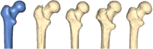
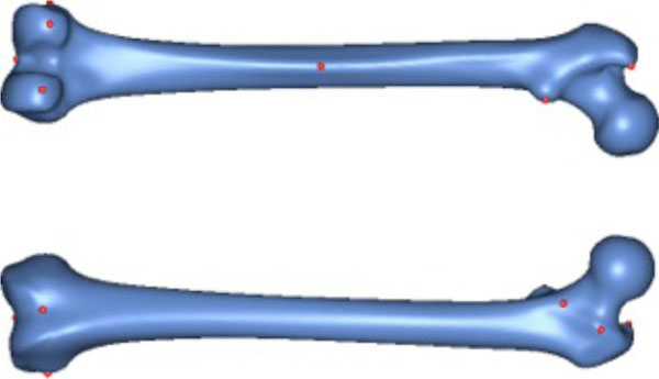
For the preparation of the study, ten salient reference points were marked on the femur template by a medical expert (see Fig. 4). Most of the points chosen have some anatomical significance (e.g. a point marking the trochanter minor). Then ten femora were randomly chosen from the database. However, samples with obvious pathological deformities were excluded. Fig. (5) displays the set of samples used.
The 10 reference points used for validation.

The 10 samples used for validation.
For the actual study 12 medically trained subjects were given the image of the bone template with the previously marked points on it and than asked to identify the corresponding points on all 10 bone samples. To compensate for intrasubject variance, every participant performed the experiment a total of three times on a weekly schedule. Intra-subject variance turned out to be 2.4 mm, measured as the average over all root mean square errors calculated for each specific point triple.
Fig. (7) displays the results of this study. The top row shows the points that were marked on the bone template and given as reference to the participants. The rows below display the distribution of the points marked by the subjects on the sample bones. In these the point to which the reference point was mapped by our algorithm is drawn in red, and the mean point of all manually marked points is drawn in blue. The smaller black dots indicate the individual points marked by the participants.
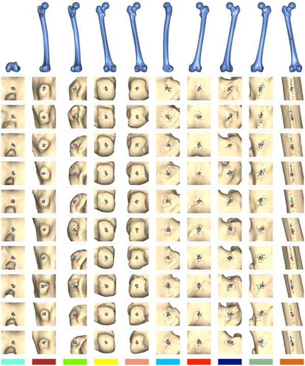
Results of the evaluation study. The algorithmically mapped point is displayed in red, the mean of the manually marked points in blue. The smaller black dots are the individual points marked by the human subjects.
Fig. (8) shows the distances between the algorithmically mapped point and the mean of the manually marked points. Fig. (9) displays the corresponding root mean square (RMS) deviations of the manually marked points, which are a measure for the uncertainty with which corresponding points were identified (the values represent the RMS of the distances of the marked points from the mean point, i.e. the distances of the black dots from the blue point in Fig. 7). As can be seen, the uncertainty varies somewhat with the location of the template point. The point with the highest locational variance is Point 10, located on the femur shaft. In this case, there is a strong anisotropy in the distribution of the points: obviously, there is a larger uncertainty along the direction of the femoral shaft rather than orthogonal to it, since the ridge on which it is located (lineaaspera) possesses saliency only in the transversal, rather than sagittal, plane. Similar charachteristics can be observed for Point 9.
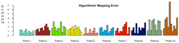
The algorithmic mapping error, grouped by point location. It’s defined as the distance between the algoritmically mapped point and the mean of the manually marked points.
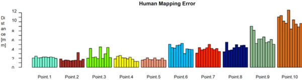
The human mapping error of the manually marked correspondences, grouped by point location. It’s defined as the root mean square (RMS) deviations of the manually marked points.
Ideally, the red and the blue points would coincide on every sample, which means that the algorithm and the human subjects (or rather, their average) agree exactly on where to place the corresponding points. As displayed in Fig. (8), the actual distances range from 1 mm to 2 mm, which seems very satisfactory for the intended use.
A natural way to assess the accuracy of the matching algorithm is to set the mapping error in relation to the RMS error of the manually marked points. Intuitively, a small RMS deviation but large mapping error would mean that the humans agree on where the point should be, but the algorithm places it apart. Likewise, a large RMS error but small mapping error would mean that the humans have no clear notion where the point should be, but the algorithm places it near their average (our assumed gold standard) nevertheless. Fig. (10) shows a combined plot of the two error values. Each point in the plot represents a unique (sample, template point) pairing, with the x axis denoting the human RMS error of this pairing, and the y axis denoting its mapping error. The shaded area represents the region in which the human RMS error exceeds the mapping error. As can be seen, nearly all points lie inside this area. Informally, this can be stated as “the uncertainty of the humans in finding point correspondences is higher than the mapping error of the algorithm”, which we take to indicate that the algorithmically detected correspondences are closer to the “gold standard” position than those obtainable from an average human.
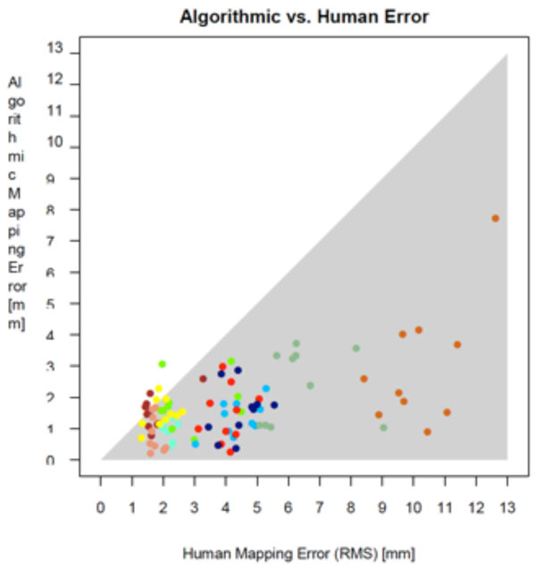
Comparison of mapping error and human error. The shaded error represents the region in which the human error exceeds the mapping error.
5. MEASUREMENT OF CCD ANGLE
As a test case scenario we set up a measurement to evaluate a measurement of the CCD angles of all women between 18 and 50 years. Our database provided 133 patients that fulfilled this criteria which were all selected and measured. Fig. (6) displays the results of this study.
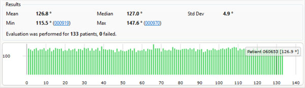
The results of an evaluation measuring the CCD angles of all women between 18 and 50 years in our database (133 samples).
CONCLUSION
We have presented a system that can be used to perform reliable morphometric measurements over anatomical databases containing a large number of individual bone samples. The system automatically detects specific anatomical landmarks, and additionally determines dense point correspondences over the entire surface of the sample bones. These features can be used as primitives for various types of constructions (such as lines, planes, etc.) based on which, in turn, various quantities can be measured (angles, lengths, etc.).
Through an extensive validation study we have shown that the correspondence mapping, which finds corresponding points over the set of all samples, performs very well in practice and produces results that are comparable or even better than those achievable by manual point mapping. Generally, the mean error between the automatic mapping and the average of human-mapped points is less than 2mm, and considerably less than the root mean square deviation of the latter. Based on this we conclude that our system is well-suited for the intended use and can produce meaningful results.
Finally a fully automated measurement of all CCD angles for 133 female patients has been performed as a test case scenario for our presented method.
CONFLICT OF INTEREST
The authors confirm that this article content has no conflict of interest.
ACKNOWLEDGEMENTS
The database of segmented bone samples used in this study was provided by Stryker Trauma GmbH, Kiel.